
Learning Objectives
- Define metapopulation, life history traits, and reproductive value
- Identify key features of an organism’s life history and how those life history traits respond to the environment and to natural selection
- Calculate population (net) reproductive rate from life tables to determine if a population is growing or shrinking
- Predict whether a population is growing, shrinking, or stable with different population growth measures (r and R0)
- Identify maximal reproductive value and explain why it changes through an organism’s lifetime
Metapopulations are populations of the same species linked together by migration (excerpted from OpenStax CNX)
A species that is ecologically linked to a specialized, patchy habitat may likely assume the patchy distribution of the habitat itself, with several different populations distributed at different distances from each other. This is the case, for example, for species that live in wetlands, alpine zones on mountaintops, particular soil types or forest types, springs, and many other comparable situations. Individual organisms may periodically disperse from one population to another, facilitating genetic exchange between the populations. This group of different but interlinked populations, with each different population located in its own, discrete patch of habitat, is called a metapopulation.
There may be quite different levels of dispersal between the constituent populations of a metapopulation. For example, a large or overcrowded population patch is unlikely to be able to support much immigration from neighboring populations; it can, however, act as a source of dispersing individuals that will move away to join other populations or create new ones. In contrast, a small population is unlikely to have a high degree of emigration; instead, it can receive a high degree of immigration. A population that requires net immigration in order to sustain itself acts as a sink. The extent of genetic exchange between source and sink populations depends, therefore, on the size of the populations, the carrying capacity of the habitats where the populations are found, and the ability of individuals to move between habitats. Consequently, understanding how the patches and their constituent populations are arranged within the metapopulation, and the ease with which individuals are able to move among them is key to describing the population diversity and conserving the species.
Life history traits and their evolution
Individuals in a population experience a life cycle of birth, growth and development, maturity to adulthood, and then decline into reproductive senescence. How energy is allocated to these different aspects of the organisms survival is called their life history, and that energy allocation generates characteristic life history traits, traits that impact survival and reproductive output: size at birth, age at maturity, size at maturity, number and size of offspring (fecundity), reproductive value, lifespan and senescence, which we will define as the decline in fecundity with age. Life History Theory explains how evolution optimizes these survival and reproductive characteristics in different populations, affecting parameters such as: how big and fast individuals grow, when they reach sexual maturity, how many offspring they have each time they reproduce, how many times the reproduce, and when they die.
Notice that survival and reproduction are “optimized,” not maximized. This is because when evolution increases one of these traits, say survival of the parent, the result is usually a decrease in some aspect of reproduction, such as number of offspring produced each year, and vice versa. This optimization generates a life-history trade-off, depicted as a negative relationship between survival and reproduction (see figure below).

The leading hypothesis for trade-offs in survival and reproduction is that energy is the limiting factor: organisms have finite energy, so if they allocate energy toward survival, then they don’t have as much available to reproduce. As a result, some organisms like the Chinook salmon reproduce only once in their short lifetime, while others such as Atlantic Cod—and humans—reproduce many times.
Selection for life history trade-offs between reproduction and survival can be related to a population’s growth rate and the environment’s carrying capacity. Recall that r is the intrinsic rate of natural increase of a population, and K is the environmental carrying capacity:
- Life history traits that maximize growth rate (live fast, die young) are said to be r-selected, and include traits like having very large numbers of offspring, relatively small body size, early sexual maturity, broad dispersal of offspring, limited parental care, and short life-span. Species with r-selected life history traits include insects, bacteria, many types of plants, and some small mammals such as rodents. These species tend to exploit ecological niches where they are not limited by carrying capacity, in part because while they produce many many offspring, each individual offspring has a low chance of survival. Their population sizes can change dramatically over short periods of time.
- Life history traits that are selected for in organisms living at densities near the environmental carrying capacity are called K-selected, and include traits which are essentially the opposite of r-selected traits: relatively small numbers of offspring, comparatively large body size, late sexual maturity, offspring which require a high degree of parental care, and longer life-span. Species with K-selected life history traits include large organisms such as many large mammals, some species of reptiles, and some species of birds. In the absence of natural disaster, disease epidemic, or other catastrophic event, the population size of these species tend to remain relatively stable and close to the maximum carrying capacity.
Regardless of whether a species has more r-selected or K-selected traits, individuals can have different likelihoods of successful reproduction at different stages of their lives. Reproductive value is the relative number of offspring that remain to be born to individuals of a given age. Reproductive value is influenced by the probability of survival as well as the probability of successful reproduction. For that reason, reproductive value is very low at birth, when the chances of death are high. From birth, reproductive value tends to increase to a maximum value at or near the onset of sexual maturity, and thereafter declines as individuals age. Natural selection acts most efficiently on age classes and life cycle stages with high reproductive value.
Life tables are a valuable tool to examine how age structure can change a population’s growth trajectory
Population demography is the study of numbers and rates in a population and how they change over time. The basic tool of demography is the life table. Life tables are an analytical tool that population ecologists use to study age-specific population characteristics such as survival, fecundity, and mortality. These data can be critical in conservation efforts (such as reintroductions or pest reductions) where ecologists would like to know how well an endangered or transplanted population is doing.
Life tables determine the number of individuals that survive from one age group to the next. Cohort life tables follow one group of individuals born at the same time, called a cohort, until the death of all individuals. This technique of demographic assessment requires key assumptions:
- The population sample of each age class is proportional to its numbers in the population
- Age-specific mortality rates remain constant during the time period, meaning that subsequent cohorts will exhibit similar pattern of birth and death.
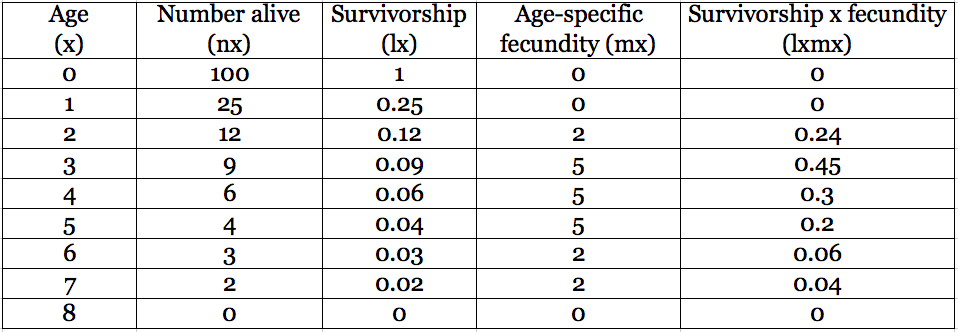
Life Table:
The first row represents the birth year of the cohort, and each subsequent row of the life table shows that same group one year older. Assuming that the unit of age (x) is years, the number alive (nx) column indicates that not all individuals survive from year to year. Survivorship converts that mortality into a proportion alive of the original cohort (lx = nx/n0). The average number of offspring born to individuals of each age is age-specific fecundity, and it cannot be calculated from other information provided in the table but instead must be estimated from data.
Here’s the best bit and the reason we bother to gather all the age-specific survivorship and fecundity information: if the assumptions (1 and 2 above) are met, then the sum of the product of survivorship and fecundity at each age gives a population growth parameter called R0 (pronounced R-nought), defined as the net reproductive rate. When R0 exceeds 1, the population is producing more offspring than it is losing from deaths. In other words, the population is growing.
- Is the population above growing, shrinking, or stable?
- At what age is fecundity maximized? Survivorship?
Because of life history trade-offs, patterns of age-specific survival are predictive of the general life history of a population. While a life table shows the survivorship in a numerical form, assessing pattern from columns of data is difficult. Instead, ecologists create survivorship curves by plotting lx versus time.
Population biologists look for three types of patterns in survivorship curves (note that the y-axis is a log scale):
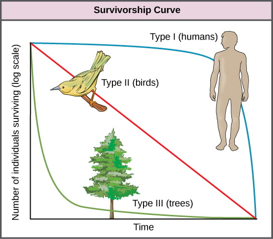
Type I curves are observed in populations with low mortality in young age classes but very high mortality as an individual ages. Type II curves represent populations where the mortality rate is constant, regardless of age. Type III curves occur in populations with high mortality in early age classes and very low mortality in older individuals. Populations displaying a Type III survivorship curve generally need to have high birth rates in order for the population size to remain constant. High birth rates ensure that enough offspring survive to reproduce, ensuring the population sustains itself. In contrast, populations characterized by a Type I survivorship curve often have low birth rates because most offspring survive to reproduce, and very high birth rates result in exponential population growth.
This video provides an overview of survivorship curves and some of the nuance in interpreting these plots:
As noted in the video, species with Type I survivorship curves tend to have K-selected traits, while species with Type III (or sometimes Type II) survivorship curves tend to have r-selected traits.
UN Sustainable Development Goal

SDG 3: Good Health and Well-being – Calculating population reproductive rates from life tables is important for understanding the demographic characteristics of a population and the potential for population growth or decline, which can impact human health and well-being. The strategies of modeling population growth can be applied to directly human populations or to the living things they consume through the conservation and management of non-human populations.
